
안녕하세요
블레이즈 테크노트의
블레이즈입니다.

지난 포스팅에서 머신러닝 지도학습 중 분류 분석 모델을 다뤘습니다.
2024.03.01 - [분류 전체보기] - 머신러닝 이론 분류모델: 로지스틱 회귀, 선형 판별 분석, k-최근접 이웃 분석
이번 포스팅에서는 해당 분석법들을 실제 데이터로 분석해보고자 합니다.
이번 분석에서 사용한 데이터는 포스팅 최하단에 업로드하겠습니다.
먼저, 필요한 라이브러리를 불러오고 데이터를 준비해보죠. 데이터는 포스팅 말미에 첨부해두었으니, 함께 확인해주세요.
import pandas as pd
import numpy as np
from time import time

import matplotlib.pyplot as plt
import seaborn as sns

from sklearn.preprocessing import OneHotEncoder
from sklearn.preprocessing import StandardScaler

from sklearn.model_selection import train_test_split
from imblearn.under_sampling import RandomUnderSampler

from sklearn.metrics import confusion_matrix, accuracy_score, recall_score, precision_score, f1_score, roc_auc_score, roc_curve, auc

import warnings
warnings.filterwarnings(action='ignore')
가장 먼저 할 일은 데이터 탐색과 전처리 과정입니다.
이 과정에서는 데이터를 살펴보고, 필요한 변환을 수행해 데이터를 모델 학습에 적합한 형태로 만들어줍니다.
해당 과정은 회귀 분석에서 진행했던 전처리 과정과 유사하니 이를 참고하셔도 좋을 것 같습니다.
2024.02.28 - [머신러닝(Machine Learning)] - 머신러닝 실습: 회귀분석 연습 1
file_path = './data_classification.csv'
df = pd.read_csv(file_path)
df.columns
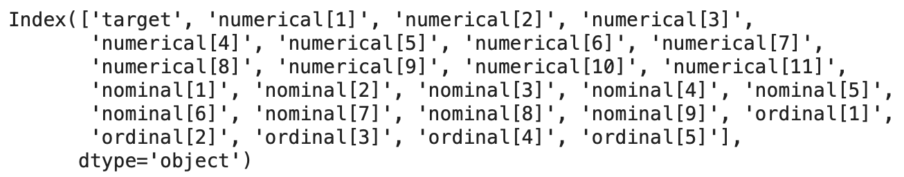
컬럼을 부르기 편하도록 그룹지어 주도록 하겠습니다.
numerical_var = ['numerical[1]', 'numerical[2]', 'numerical[3]',
       'numerical[4]', 'numerical[5]', 'numerical[6]', 'numerical[7]',
       'numerical[8]', 'numerical[9]', 'numerical[10]', 'numerical[11]']
nominal_var = ['nominal[1]', 'nominal[2]', 'nominal[3]', 'nominal[4]', 'nominal[5]',
       'nominal[6]', 'nominal[7]', 'nominal[8]', 'nominal[9]']
ordinal_var = ['ordinal[1]', 'ordinal[2]', 'ordinal[3]', 'ordinal[4]', 'ordinal[5]']
targert_var = ['target']
nominal 변수의 경우 아래와 같이 0 또는 1 이므로 카테고리 타입으로 타입을 변환해주도록 하겠습니다.
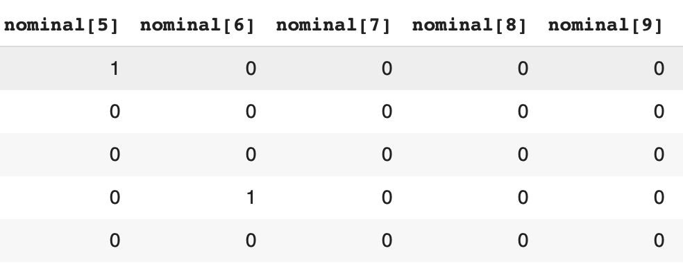
 df[nominal_var] = df[nominal_var].astype('category')
 df[nominal_var].dtypes
통계량 확인을 해주겠습니다.
df.describe()
category 타입으로 변환된 변수의 경우 통계량 계산에서 자동으로 제외됩니다.
df.isnull().sum(axis=0)

당연히 결측치가 있겠죠?
df = df.dropna(axis=0)결측치 제거를 해줬습니다.
이번 데이터 분석의 핵심은 명목형 변수를 원-핫 인코딩으로 처리하고,
순서형 변수에 대한 스케일링을 진행하는 것입니다.
명목형 변수의 원-핫 인코딩은 데이터를 모델이 이해할 수 있는 형태로 변환하는 중요한 단계입니다.
from sklearn.preprocessing import OneHotEncoder
ohe_encoding = pd.get_dummies(df[nominal_var])
ohe_var = ohe_encoding.columns
df = df.drop(nominal_var, axis=1) #카테고리형 변수들 제거
df = pd.concat([df, ohe_encoding],axis=1) #원핫인코딩 변수 추가
다음으로는 순서형 변수들을 처리해줄 차례입니다.
순서형 변수는 1,2,3,4,5 이런 값들이 있는데요
다른 변수의 1,2,3,4,5와 첫째 둘째 셋째 넷째의 의미가 조금 다르겠죠?
이러한 맥락을 담는다고 생각하시면 될 것 같습니다.
from sklearn.preprocessing import MinMaxScaler

mm_scaler = MinMaxScaler()
mm_scaler.fit(df[ordinal_var])
df[ordinal_var] = mm_scaler.transform(df[ordinal_var])
df[ordinal_var].head()
MinMaxScaler로 스케일을 바꿔주었어요

다음으로 트레이닝 테스트 데이터 분리를 해보도록 하겠습니다.
from sklearn.model_selection import train_test_split

target = df['target'] # 종속 변수
data = df.loc[:,(c != 'target' for c in df.columns)] # 독립변수

### train test split 수행
tr_x, te_x, tr_y, te_y = train_test_split(data, target, test_size = 0.05, random_state = 0, shuffle=True)
이번에는 95:5 의 비율로 트레인 테스트 스플릿을 진행했습니다.
from imblearn.under_sampling import RandomUnderSampler

sns.histplot(tr_y)
plt.show()
print('정상 검진 수(비율): {}({:.1f}%)'.format(len(tr_y[tr_y==0]),len(tr_y[tr_y==0])/len(tr_y)*100))
print('환자 수(비율):  {}({:.1f}%)'.format(len(tr_y[tr_y==1]),len(tr_y[tr_y==1])/len(tr_y)*100))
이번 데이터의 경우 데이터 자체에 불균형이 있습니다.
실제 환자의 비율이 7%이네요.
다만 이렇게 불균형된 데이터로 학습을 할 경우 학습이 제대로 이뤄지지 않을 경우가 있습니다.
이럴 때는 불균형을 없애주기 위해서 많은 데이터를 없애던지
적은 데이터를 증폭시켜야 합니다.
데이터의 불균형 문제를 해결하기 위해 RandomUnderSampler를 사용하여 클래스 간 균형을 맞춰주었습니다.
under_tr_x, under_tr_y = RandomUnderSampler(random_state=0).fit_resample(tr_x, tr_y)

under_tr_x = pd.DataFrame(under_tr_x, columns=tr_x.columns)

sns.histplot(under_tr_y)
plt.show()
print('정상 검진 수(비율): {}({:.1f}%)'.format(len(under_tr_y[under_tr_y==0]),len(under_tr_y[under_tr_y==0])/len(under_tr_y)*100))
print('환자 수(비율):  {}({:.1f}%)'.format(len(under_tr_y[under_tr_y==1]),len(under_tr_y[under_tr_y==1])/len(under_tr_y)*100))

학습 데이터의 불균형을 RandomUnderSampler로 균형을 맞췄습니다.
데이터 불균형을 처리하는 방법은 다음의 두가지가 있습니다.
- Over sampling : 소수의 클래스에 속한 데이터 셋의 샘플 수를 다수의 클래스에 속한 샘플 수에 맞춰서 증가시키는 기법입니다. 이는 없는 샘플을 만드는 것이기 때문에 사용 시에 유의를 해야함.
- Under sampling : 다수의 클래스에 속한 데이터 셋의 샘플 수를 소수의 클래스에 속한 샘플 수에 맞춰서 샘플링 하는 기법
참고 : https://imbalanced-learn.org/stable/under_sampling.html#under-sampling
3. Under-sampling — Version 0.12.0
3. Under-sampling One way of handling imbalanced datasets is to reduce the number of observations from all classes but the minority class. The minority class is that with the least number of observations. The most well known algorithm in this group is rand
imbalanced-learn.org
이후, 수치형 변수에 대해 정규화를 수행하였습니다. 정규화는 모델의 성능을 최적화하기 위해 필수적인 단계입니다.
numerical 변수에 대해서만 StandardScaler를 활용해 정규화를 진행했습니다.
from sklearn.preprocessing import StandardScaler

sns.barplot(x=numerical_var, y=tr_x[numerical_var].mean(axis=0))
plt.xticks(rotation = 300)
plt.show()

s_scaler = StandardScaler()
s_scaler.fit(tr_x[numerical_var])
tr_standardization = s_scaler.transform(under_tr_x[numerical_var])
te_standardization = s_scaler.transform(te_x[numerical_var])


scaled_tr_x = np.concatenate([tr_standardization, under_tr_x[ordinal_var], under_tr_x[ohe_var].values],axis=1)
scaled_te_x = np.concatenate([te_standardization, te_x[ordinal_var], te_x[ohe_var].values],axis=1)
정규화한 numerical 변수와 undersampling을 진행한 순서형 변수, 원핫인코딩 처리한 명목형 변수를 concatenate 했습니다.
# 트레이닝 셋
pd.DataFrame(scaled_tr_x, columns=numerical_var+ordinal_var+ohe_var.tolist()).describe()

# 테스트 셋
pd.DataFrame(scaled_te_x, columns=numerical_var+ordinal_var+ohe_var.tolist())

스케일링이 잘 된 것 같죠?
모델 학습에 앞서 평가 지표부터 만들고 시작하도록 하겠습니다.
def get_clf_eval(y_test, y_pred, y_prob):
    confusion = confusion_matrix(y_test, y_pred)
    accuracy = accuracy_score(y_test, y_pred)
    precision = precision_score(y_test, y_pred)
    recall = recall_score(y_test, y_pred)
    F1 = f1_score(y_test, y_pred)
    AUC = roc_auc_score(y_test, y_prob[:,1])

    print('오차행렬:\n', confusion)
    print('\n정확도(Accuracy): {:.4f}'.format(accuracy))
    print('정밀도(Precision): {:.4f}'.format(precision))
    print('재현율(Recall): {:.4f}'.format(recall))
    print('F1: {:.4f}'.format(F1))
    print('AUC: {:.4f}'.format(AUC))
def get_clf_roc_curve(y_test, y_prob):
    fpr, tpr, thresholds = roc_curve(y_test, y_prob[:,1])
    roc_auc = auc(fpr, tpr)
    plt.plot(fpr, tpr, 'b', label = 'AUC = %0.4f' % roc_auc)
    plt.legend(loc = 'lower right')
    plt.plot([0, 1], [0, 1],'r--')
    plt.xlim([0, 1])
    plt.ylim([0, 1])
    plt.title("ROC curve")
    plt.ylabel('True Positive Rate')
    plt.xlabel('False Positive Rate')
    plt.show()
평가지표를 먼저 만들었습니다.
정확도, 정밀도, 재현율, F1, AUC 를 통해 평가를 하려고 합니다.
ROC 그래프도 그려보도록 하겠습니다.
평가지표에 대한 개념 설명 :
다음 포스팅에서는 실제로 모델을 학습해보도록 하겠습니다.
감사합니다.
블레이즈 테크 노트.
'머신러닝(Machine Learning)' 카테고리의 다른 글
| 머신러닝 실습: 분류분석 연습2 (0) | 2024.03.03 |
|---|---|
| 머신러닝 실습: 회귀분석 연습2 (0) | 2024.02.29 |
| 머신러닝 실습: 회귀분석 연습 1 (0) | 2024.02.28 |
| 머신러닝 이론 선형회귀모델: Ridge, Lasso, Elastic Net (0) | 2024.02.26 |
| 머신러닝 기초_pandas, matplotlib.pyplot 활용하기 (0) | 2024.02.25 |


